Standard pipeline: analyzing 5K PBMC dataset from 10X genomics

Introduction

In this tutorial we will analyze single-cell ATAC-seq data from Peripheral blood mononuclear cells (PBMCs).

Import library and environment setup

import snapatac2 as snap

snap.__version__

'2.5.0dev2'

To start, we need to download a fragment file. This can be achieved by calling the function below.

# Input files
fragment_file = snap.datasets.pbmc5k()
fragment_file

PosixPath('/home/zhangkaiLab/zhangkai33/.cache/snapatac2/atac_pbmc_5k.tsv.gz')

A fragment file refers to a file containing information about the fragments of DNA that are accessible and have been sequenced. Here are more information about the Fragment File.

If you do not have a fragment file for your experiment, you can make one from a BAM file, see pp.make_fragment_file().

Preprocessing

We begin data preprocessing by importing fragment files and calculating basic quality control (QC) metrics using the pp.import_fragments() function.

This function compresses and stores the fragments in an AnnData object for later usage(To learn more about SnapATAC2’s anndata implementation, click here). During this process, various quality control measures, such as TSS enrichment and the number of unique fragments per cell, are computed and stored in the anndata as well.

When the file argument is not specified, the AnnData object is created and stored in the computer’s memory. However, if the file argument is provided, the AnnData object will be backed by an hdf5 file. In “backed” mode, pp.import_fragments() processes the data in chunks and streams the results to the disk, using only a small, fixed amount of memory. Therefore, it is recommended to specify the file parameter when working with large datasets and limited memory resources. Keep in mind that analyzing data in “backed” mode is slightly slower than in “memory” mode.

In this tutorial we will use the backed mode. To learn more about the differences between these two modes, click here.

%%time
data = snap.pp.import_fragments(
    fragment_file,
    chrom_sizes=snap.genome.hg38,
    file="pbmc.h5ad",  # Optional
    sorted_by_barcode=False,
)
data

CPU times: user 6min 32s, sys: 9.15 s, total: 6min 41s
Wall time: 3min 17s

AnnData object with n_obs x n_vars = 14232 x 0 backed at 'pbmc.h5ad'
    obs: 'n_fragment', 'frac_dup', 'frac_mito'
    uns: 'reference_sequences'
    obsm: 'fragment_paired'

pp.import_fragments() computes only basic QC metrics like the number of unique fragments per cell, fraction of duplicated reads and fraction of mitochondrial read. More advanced metrics can be computed by other functions.

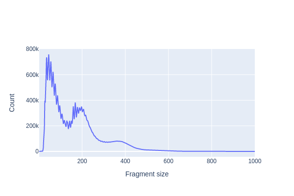
We first use pl.frag_size_distr() to calculate and plot the size distribution of fragments in this dataset. The typical fragment size distribution in ATAC-seq data exhibits several key characteristics:

1. Nucleosome-Free Region (NFR): The majority of fragments are short, typically around 80-300 base pairs (bp) in length. These short fragments represent regions of open chromatin where DNA is relatively accessible and not bound to nucleosomes. These regions are often referred to as nucleosome-free regions (NFRs) and correspond to regions of active transcriptional regulation.

2. Mono-Nucleosome Peaks: There is often a peak in the fragment size distribution at around 147-200 bp, which corresponds to the size of a single nucleosome wrapped DNA. These fragments result from the cutting of DNA by the transposase enzyme when it encounters a nucleosome, causing the DNA to be protected and resulting in fragments of the same size.

3. Di-Nucleosome Peaks: In addition to the mono-nucleosome peak, you may also observe a smaller peak at approximately 300-400 bp, corresponding to di-nucleosome fragments. These fragments occur when transposase cuts the DNA between two neighboring nucleosomes.

4. Large Fragments: Some larger fragments, greater than 500 bp in size, may be observed. These fragments can result from various sources, such as the presence of longer stretches of open chromatin or technical artifacts.

snap.pl.frag_size_distr(data, interactive=False)

2023-10-08 13:50:58 - INFO - Computing fragment size distribution...

The plotting functions in SnapATAC2 can optionally return a plotly Figure object that can be further customized using plotly’s API. In the example below, we change the y-axis to log-scale.

fig = snap.pl.frag_size_distr(data, show=False)
fig.update_yaxes(type="log")
fig.show()

Another important QC metric is TSS enrichment (TSSe). TSSe in ATAC-seq data implies that there is an increased accessibility or fragmentation of chromatin around the transcription start sites of genes. This is often indicative of open and accessible promoter regions, which are typically devoid of nucleosomes and are involved in active gene transcription.

Researchers often use TSS enrichment as a quality control metric in these assays. If there is a clear and pronounced enrichment of reads or signal around TSS regions, it suggests that the experiment has captured relevant genomic features and is likely to yield biologically meaningful results. Conversely, a lack of TSS enrichment may indicate issues with the experiment’s quality or data processing.

TSSe scores of individual cells can be computed using the metrics.tsse() function.

%%time
snap.metrics.tsse(data, snap.genome.hg38)

CPU times: user 1min 49s, sys: 2.45 s, total: 1min 52s
Wall time: 23.6 s

To identify usable/high-quality cells, we can plot TSSe scores against number of unique fragments for each cell.

snap.pl.tsse(data, interactive=False)

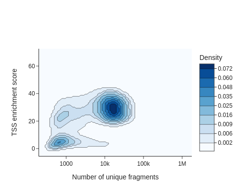
The cells in the upper right represent valid or high-quality cells, whereas those in the lower left represent low-quality cells or empty droplets. Based on this plot, we decided to set a minimum TSS enrichment of 10 and a minimum number of fragments of 5,000 to filter the cells.

%%time
snap.pp.filter_cells(data, min_counts=5000, min_tsse=10, max_counts=100000)
data

CPU times: user 20.2 s, sys: 929 ms, total: 21.2 s
Wall time: 21.3 s

AnnData object with n_obs x n_vars = 4564 x 0 backed at 'pbmc.h5ad'
    obs: 'n_fragment', 'frac_dup', 'frac_mito', 'tsse'
    uns: 'reference_sequences', 'frag_size_distr'
    obsm: 'fragment_paired'

We next create a cell by bin matrix containing insertion counts across genome-wide 500-bp bins.

%%time
snap.pp.add_tile_matrix(data)

CPU times: user 49.8 s, sys: 2 s, total: 51.8 s
Wall time: 25.9 s

Next, we perform feature selection using pp.select_features(). The result is stored in data.var['selected'] and will be automatically utilized by relevant functions such as pp.scrublet() and tl.spectral().

The default feature selection algorithm chooses the most accessible features. The n_features parameter determines the number of features or bins used in subsequent analysis steps. Generally, including more features improves resolution and reveals finer details, but it may also introduce noise. To optimize results, experiment with the n_features parameter to find the most appropriate value for your specific dataset.

Additionally, you can provide a filter list to the function, such as a blacklist or whitelist. For example, use pp.select_features(data, blacklist='blacklist.bed').

snap.pp.select_features(data, n_features=250000)

2023-10-08 13:52:32 - INFO - Selected 250000 features.

Doublet removal

Here we apply a customized scrublet algorithm to identify potential doublets. Calling pp.scrublet() will assign probabilites of being doublets to the cells. We can then use pp.filter_doublets to get the rid of the doublets.

%%time
snap.pp.scrublet(data)

2023-10-08 13:52:39 - INFO - Simulating doublets...
2023-10-08 13:52:40 - INFO - Spectral embedding ...
2023-10-08 13:53:42 - INFO - Calculating doublet scores...

CPU times: user 1min 29s, sys: 1min 3s, total: 2min 32s
Wall time: 1min 16s

This line does the actual filtering.

snap.pp.filter_doublets(data)
data

2023-10-08 13:53:49 - INFO - Detected doublet rate = 2.936%

AnnData object with n_obs x n_vars = 4430 x 6062095 backed at 'pbmc.h5ad'
    obs: 'n_fragment', 'frac_dup', 'frac_mito', 'tsse', 'doublet_probability', 'doublet_score'
    var: 'count', 'selected'
    uns: 'reference_sequences', 'scrublet_sim_doublet_score', 'doublet_rate', 'frag_size_distr'
    obsm: 'fragment_paired'

Dimension reduction

To calculate the lower-dimensional representation of single-cell chromatin profiles, we employ spectral embedding for dimensionality reduction. The resulting data is stored in data.obsm['X_spectral']. Comprehensive information about the dimension reduction algorithm we utilize can be found in the algorithm documentation.

%%time
snap.tl.spectral(data)

CPU times: user 36.8 s, sys: 43 s, total: 1min 19s
Wall time: 24.9 s

We then use UMAP to embed the cells to 2-dimension space for visualization purpose. This step will have to be run after snap.tl.spectral as it uses the lower dimesnional representation created by the spectral embedding.

%%time
snap.tl.umap(data)

/storage/zhangkaiLab/zhangkai33/software/micromamba/lib/python3.10/site-packages/tqdm/auto.py:21: TqdmWarning:

IProgress not found. Please update jupyter and ipywidgets. See https://ipywidgets.readthedocs.io/en/stable/user_install.html

/storage/zhangkaiLab/zhangkai33/software/micromamba/lib/python3.10/site-packages/umap/umap_.py:1943: UserWarning:

n_jobs value -1 overridden to 1 by setting random_state. Use no seed for parallelism.

CPU times: user 26.4 s, sys: 1.05 s, total: 27.4 s
Wall time: 31.8 s

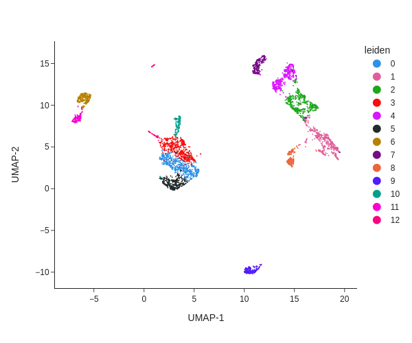
Clustering analysis

We next perform graph-based clustering to identify cell clusters. We first build a k-nearest neighbour graph using snap.pp.knn, and then use the Leiden community detection algorithm to identify densely-connected subgraphs/clusters in the graph.

%%time
snap.pp.knn(data)
snap.tl.leiden(data)

CPU times: user 892 ms, sys: 75.1 ms, total: 968 ms
Wall time: 1.05 s

snap.pl.umap(data, color='leiden', interactive=False, height=500)

The plot can be saved to a file using the out_file parameter. The suffix of the filename will used to determined the output format.

snap.pl.umap(data, color='leiden', show=False, out_file="umap.pdf", height=500)
snap.pl.umap(data, color='leiden', show=False, out_file="umap.html", height=500)

Cell cluster annotation

Create the cell by gene activity matrix

Now that we have the cell clusters, we will try to annotate the clusters and assign them to known cell types. To do this, we need to compute the gene activities first for each cell using the pp.make_gene_matrix function.

Just like pp.import_data, pp.make_gene_matrix allows you to provide an optional file name used to store the AnnData object. To demo the in-memory mode of AnnData, we will not provide the file parameter this time.

%%time
gene_matrix = snap.pp.make_gene_matrix(data, snap.genome.hg38)
gene_matrix

CPU times: user 2min 54s, sys: 3.68 s, total: 2min 58s
Wall time: 41.5 s

/storage/zhangkaiLab/zhangkai33/software/micromamba/lib/python3.10/site-packages/anndata/_core/anndata.py:121: ImplicitModificationWarning:

Transforming to str index.

AnnData object with n_obs × n_vars = 4430 × 60606
    obs: 'n_fragment', 'frac_dup', 'frac_mito', 'tsse', 'doublet_probability', 'doublet_score', 'leiden'

Imputation

The cell by gene activity matrix is usually very sparse. To ease the visulization and marker gene identification, we use the MAGIC algorithm to perform imputation and data smoothing. The subsequent steps are similar to those in single-cell RNA-seq analysis, we therefore leverage the scanpy package to do this.

Since we have stored the gene matrix in in-memory mode, we can directly pass it to scanpy. If the AnnData object is in backed mode, you need to convert it to an in-memory representation using the .to_memory() method.

We first perform gene filtering, data normalization, data transformation, and then call the sc.external.pp.magic function to complete the imputation. For this to work, you need to install the magic-impute package: pip install magic-impute.

import scanpy as sc

sc.pp.filter_genes(gene_matrix, min_cells= 5)
sc.pp.normalize_total(gene_matrix)
sc.pp.log1p(gene_matrix)

%%time
sc.external.pp.magic(gene_matrix, solver="approximate")

CPU times: user 1min 16s, sys: 13.4 s, total: 1min 30s
Wall time: 58.8 s

# Copy over UMAP embedding
gene_matrix.obsm["X_umap"] = data.obsm["X_umap"]

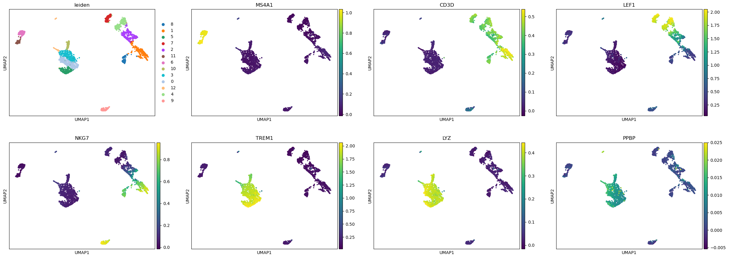
We can now visualize the gene activity of a few marker genes.

marker_genes = ['MS4A1', 'CD3D', 'LEF1', 'NKG7', 'TREM1', 'LYZ', 'PPBP']
sc.pl.umap(gene_matrix, use_raw=False, color=["leiden"] + marker_genes)

/storage/zhangkaiLab/zhangkai33/software/micromamba/lib/python3.10/site-packages/scanpy/plotting/_tools/scatterplots.py:391: UserWarning:

No data for colormapping provided via 'c'. Parameters 'cmap' will be ignored

Close AnnData objects

When the AnnData objects are opened in backed mode, they will be synchronized with the underlying HDF5 files, which means there is no need to manually save the results during the analysis and the files are always up to date. As a side effect, it is important to close every backed AnnData object before shutdown the Python process to avoid HDF5 file corruptions!

data.close()
data

Closed AnnData object

Also, remember to save any in-memory AnnData objects.

gene_matrix.write("pbmc5k_gene_mat.h5ad", compression='gzip')

Now it is safe to close and shutdown the notebook! Next time you can load the results using data = snap.read("pbmc.h5ad").

What’s next?

• Cell type annotation

• Differential peak and motif analysis